I’ve just released version 4.0 of simplex-noise.js. Based on user feedback the new version supports tree shaking and cleans up the API a bit. As a nice little bonus, it’s also about 20% - 30% faster.
It also removes the bundled PRNG to focus the library down to one thing - providing smooth noise in multiple dimensions.
The API Change
The following bit of code should illustrate the changes to the API well:
// 3.x forces you to import everything at once
import SimplexNoise from 'simplex-noise';
const simplex = new SimplexNoise();
const value2d = simplex.noise2D(x, y);
// 4.x allows you to import just the functions you need
import { createNoise2D } from 'simplex-noise';
const noise2D = createNoise2D();
const value2d = noise2D(x, y);
Tree shaking
Thew new API enables javascript bundler to perform tree shaking.
Essentially dead code removal based on imports and exports.
Tree shaking reduces the size of bundled javascript by leaving out code that isn’t used. As author of a library it enables me to worry less about the bundle size impact of features that might not be used by the majority of users.
A little demo to celebrate
The release of 4.0 and getting over 1’000 stars on github was a good excuse to write a little demo to celebrate.
For some extra fun I’ve decided to constrain myself to code a bit like I did in 2010 again. Canvas 2d only. No WebGL. :)
The performance implications of that decision are pretty terrible but it’s not like the world needs a demo to proof that quads can be rendered more quickly anyways. ;)
The demo uses 2 octaves of 2d noise from simplex-noise.js in a FBM configuration. The noise is then modulated with a few sine waves to create a twisting road, mountains and more flat plains.
At the highest resolutions the demo is pushing 4096 quads/frame! A bit more than the SuperFX Chip on SNES could handle. ;)
If you are interested in more details the code is available on github.
The future
With tree shaking reducing the impact of rarely used code it could be fun to add a few more features to simplex-noise.js in the future. A few ideas that come to mind are:
Noise with a controllable period (aka tileable noise)
Noise in 1D
More random noise using a (better) hash function like xxhash
A little while ago I came across an interesting post on reddit on how a wood displacement map can enhance the look of 3D prints.
Just a bit before I also played with the fuzzy skin feature in prusa slicer 2.4.
That made me wonder whether the wood effect could be achieved directly in the slicer by tweaking the fuzzy skin feature.
I had a quick look at the prusa slicer source and it looked like it would be fairly easy to add.
To prototype the idea and gauge whether there is any interest in it I decided that it would be best to create a little web app using three.js.
For the effect to just work I had to avoid uv maps.
Instead I’m using a basic volumetric (3d) procedural wood texture
derived from sine waves and a bit of noise.
Preliminary results
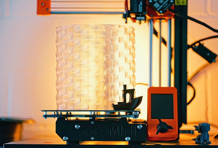
To test the process I designed and printed a very simple phone stand and a 3D benchy using Polymaker PolyWood filament.
Benchy and phone stand on the prusa mini.
The phone stand lit by the sun.
Known issues
When processing STL files I first tesselate the geometry and then perform the displacement mapping.
Luckily there is a simple tesselator built into three.js which I could use. Unfortunately it creates t-juction (when running out of iterations).
The displacement mapping can also lead to self intersections.
I also included a process for directly modifying G-code to test how
this process could work when integrated into the slicer.
When processing g-code I simply look for the perimeter comments inserted by prusa slicer and modify the G1 movement commands.
Moves are currently not sub divided.
So the tool is far from perfect but I’m quite happy with the results I got from it so far.
Possible future work
If there is enough interest in texturing features like this I think it would be pretty cool to integrate them directly into the slicer.
Obviously the wood effect isn’t the only pattern that could be achieved with this approach. Playing with different textures could definitely be fun as well.
I enjoy the swirly blur in the out of focus regions that certain lenses like the historic Petzval produce.
This effect is also known is swirly bokeh.
Just not quite enough to own such a lens myself (yet).
Instead I’ve chosen to emulate it by 3d printing a special lens hood
for my Sony FE 55/1.8 lens.
How to get swirly bokeh with a lens hood
A similar effect to the one produced by these old lenses can be achieved using a lenshood
that restricts the paths light can take into the lens.
The swirly effect is essentially created by the opening of the lens hood being to small.
This creates mechanical vignetting (also known as cat’s eye bokeh),
blocking part of the light from hitting the sensor.
The light coming from the left (yellow, orange) is partially blocked by the lens hood (black) before hitting the lens (blue) and finally the sensor on the right (black).
In most lenses that produce this effect the vignetting happens somewhere inside the lens but the effect it has is similar.
3D printing a swirly bokeh lens hood
To test out how well this works in practice I modelled such a restrictive lens hood in freecad.
Preview of the 3D print.
Finished product.
Definitely not the cleanest print but at a material cost of about 20 cents (EU/US) and a print time of about 15 minutes it’s well worth it.
Results
Crop of the top right corner of some city lights at night.
Want to make your own?
I’ve thrown the source files up in a github repo for you to use jwagner/swirly-lens-hoods.
With that said, I’m a very inexperienced CAD user and in this case didn’t even try to create something clean.
If you can you might be better of just remodelling it to fit your own lens rather than trying to adapt it.
I didn’t have any lamp shades in my appartment since moving out from my parents place.
I’ve decided to change that and have some fun while doing it by building a generator for lamp shades.
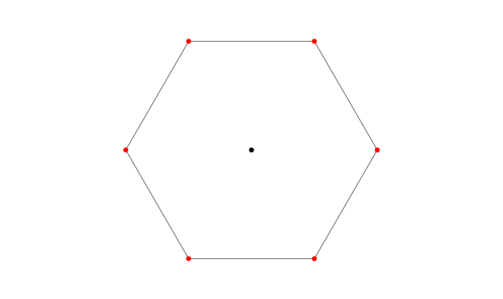
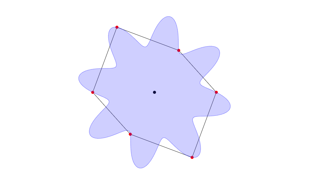
I’ve started by generating n-gons. A hexagon in this example.
In order to make the result a bit more visually appealing I then
modulated the distance from the center (radius) of each vertex
using a sine wave. This results in some interesting shapes due to aliasing.
To move into the third dimension I extrude the shape and shift the
phase of the sine wave a bit in order to twist the resulting shape.
3D Printed results
Here is what one of the models looks like in the real world.
3D printed in vase mode (as a single spiral of extruded plastic)
out of PETG using a 0.8mm nozzle.
I first learned about the fourier transform at about the same time I started to play guitar. So obviously the first idea that came to my mind at that time was to build a tuner to tune my new guitar. While I eventually got it to work the accuracy was terrible so it never ended up seeing the light of the day.
Fast forward a bit over a decade. It’s 2020 and we are fighting a global pandemic using social distancing.
I obviously tried to find ways to directly address the issue with code but in the end there is only so much that can be done on that front and a lot of really clever people on it already.
So rather than coming up with another well intended but flawed design of a mechanical ventilator I decided to revisit this old project of mine. :)
So what’s in it?
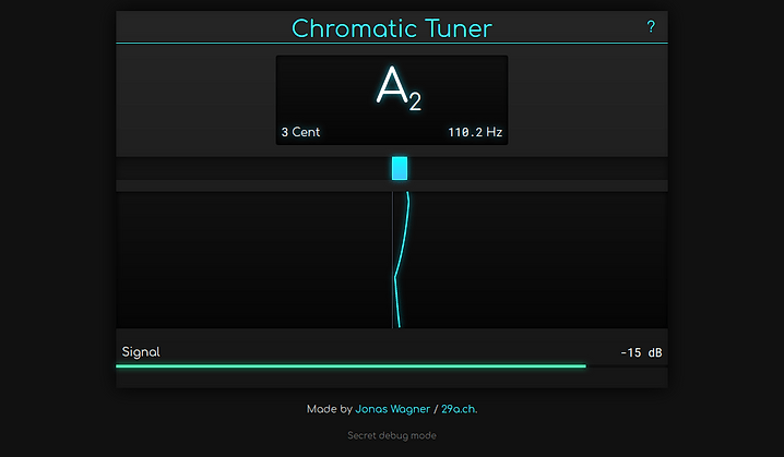
The tuner has been built with a whole lot of web tech like getUserMedia to access the microphone, WebAudio to get access to the audio data from the microphone as well as web workers to make it a bit faster. Framework wise I used React and TypeScript.
With that out of the way, the rest of the article will focus on the algorithm that makes the whole thing tick.
Disclaimer
In the following sections I will oversimplify a lot of things for the sake of accessibility and brevity.
If you already have a solid understanding of subject please excuse my oversimplifications.
If you don’t keep in mind that there is a lot more to learn and understand than what I will touch on in this description.
If you want to go deeper I highly recommend reading the papers by Philip McLeod et al. mentioned at the end. They formed the basis of this tuner.
Going beyond the fourier transform
Initially I decided to resume this project from where I stopped years ago, by doing a straight fourier transform on the input and then selecting the first significant peak (by magnitude).
The naive spectrum approach of course still works as badly as it did back then.
In slightly oversimplified terms the frequency resolution of the discrete short-time fourier transform is sample rate divided by window size.
So taking a realistic sample rate of 48000 Hz and a (comparably large) window size of 8192 samples we arrive at a frequency resolution of about 6 Hz.
The low E of a guitar in standard tuning is at ~82 Hz. Add 6 Hz and you are already past F.
We need at least 10x that to build something resembling a tuner.
In practice we should aim for a resolution of approximately 1 cent or about 100x the resolution we’d get from the straight fourier transform aproach.
There are approaches to improve the accuracy of this approach a bit, in fact we’ll meet one of them a bit later on in a different context.
For now let’s focus on something a bit simpler.
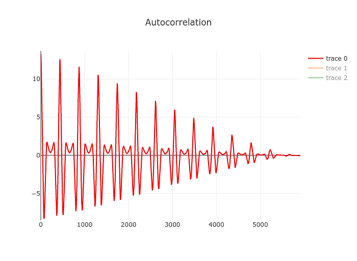
Auto correlation
Compared to the fourier transform autocorrelation is fairly simple to explain.
In essence it’s a measure of how similar a signal is to a shifted version of itself. This nicely reflect the frequency, or rather period of the signal we
are trying to determine.
In a bit more concrete terms it’s the product of the signal and a time shifted version of the signal.
In simplistic Javascript that could look a bit like this:
function autoCorrelation(signal) {
  const output = [];
  for(let lag = 0; lag < signal.length; lag++) {
    for(let i = 0; i + lag < signal.length; i++) {
      output[lag] += signal[i]*signal[i+lag]
    }
  }
  return output;
}
The result will look a bit like this:
Just by eyeballing it you can tell that it’s going to be easier to find the first significant of the autocorrelation compared to the spectrum yielded by the fourier transform above. Our resolution also changed a bit, this time we are measuring the period of the signal. Our resolution is limited by the sample rate of the signal. So to take the example above the period of a 82 Hz signal is 48000/82 or 585 samples. Being off by a sample we’d end up at 82.19 Hz. Not great but at least it’s still an E. At higher frequencies things will start to look different of course but for our purposes that’s a good point to start.
Now that we have the graph above we’ll need a robust way of determining the first significant peak in it, which hopefully will also be the perceived fundamental frequency of the tone we are analysing.
We’ll do this in two steps, first we will find all the peaks after the initial zero crossing. We can do this by just looping over the signal and keeping track of the highest value we’ve seen and it’s offset. Once the current value drops bellow 0 we can add it to the list of peaks and reset our maximum.
From this list we’ll now pick the first peak which is bigger than the highest peak multiplied by some tolerance factor like 0.9.
At this point we have a basic tuner. It’s not very robust. It’s not very fast or accurate but it should work.
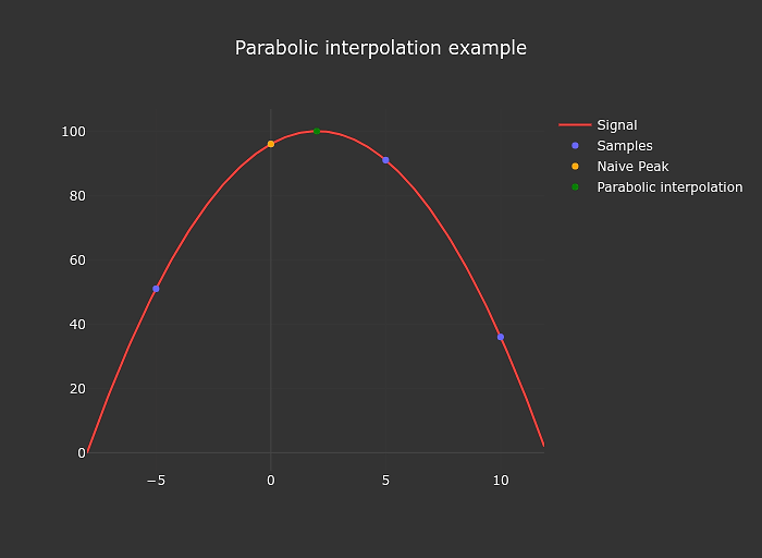
Improving accuracy
The autocorrelation algorithm mentioned above is evaluated at descrete steps matching the samples of the audio input, that limits our accuracy.
We can easily improve on this a bit by interpolating.
I use parabolic interpolation in my tuner.
The implementation of this is also extremely simple
function parabolicPeakInterpolation(a, b, c) {
  const denominator = a - 2 * b + c;
  if (denominator === 0) return 0;
  return (a - c) / denominator / 2;
}
Improving reliability
So far everything went smoothly. I had a reasonably accurate tuner for as long
as I fed it a clean signal (electric guitar straight into a nice interface).
For some reason I also wanted to get this to work using much more dirty signals
from something like a smartphone microphone.
At this stage I spend quite a bit of time implementing and evaluating various noise reduction techniques like simple filters and variations on spectral subtraction. In the end their main benefit was in being able to reduce 50/60 Hz hum but the results were still miserable.
So after banging my head against the wall for a little while I embraced a bit of a paradigm shift and gave up on trying to find a magical filter that would give me a clean signal to feed the pitch detection algorithm.
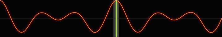
Onset Locking
I now use the brief moment right after the note has been plucked to get a decent initial guess of the note being played. This is possible because the initial attack fo the note is fairly loud resulting in a decent signal to noise ratio.
I then use this initial guess to limit the window in which I look for the peak in the auto correlation caused by the note and combine the various measurements using a simple kalman filter.
I named the scheme onset locking in my code, but I’m certain it’s not a new idea.
Making it fast
I hope the O(n²) loop in the auto correlation section made you cringe a bit.
Don’t do it that way. Both basic auto correlation and McLeods take on it (after applying a bit of basic algebra) can be accelerated using the fast fourier transform.
Good bye n squared, hello n log n. :)
Even with the relatively slow FFT implementation I’m using the speed up is between 10 and 100x. So the opimization is definitely worth doing in practice as well.
I’m also using web workers to get the calculations off the main thread and
while at it also parallelized.
The result is that the tuner runs fast enough even on my aging Galaxy S7.
What is left to do
Performance in noisy environment is still bad. Using the microphone of a macbook the tuner barely works, if the fan spins up a bit too loudly it will fail completely.
I’d definitely like to improve this in the future but I also have the suspicion that it won’t be trivial, at least without making additional assumptions about the instrument being tuned.
Another front would be to add alternative tunings, and maybe even allow custom tunings. That should be relatively easy to do but I don’t currently have any use for it.
During the past two years I’ve had the occasional pleasure of riding my motorcycles on race tracks.
While I’m still far away from being fast I really enjoy working on my riding.
This led me to considering different data recording and analysis solutions.
A bit down the line I realized that the GoPro cameras I already owned actually contain
a surprisingly good GPS unit recording data at 18hz.
To make things even better GoPro also documented their meta data format and even published
a parser for it on GitHub.
I was very curious how far I could get with that data and started to play around with it.
Many hours and experiments later I somehow ended up with my own analysis software and filters tuned for
the camera data.
For filtering the data I wrote a little library for kalman filters in TypeScript. The Kalman Filter book by Roger Labbe helped a lot in learning about the topic.
I highly recommend it if you want to dive into the topic yourself.
In addition to the obvious line plots of speed, acceleration and lean angles I also implemented a detailed map and
what I call a G Map.
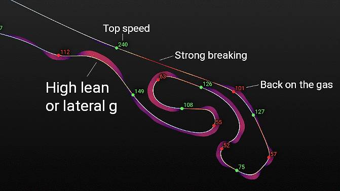
Lap Map
The lap map shows the line, speeds, breaking points and g forces in a spatial context.
I especially like the shaded areas in the corners. They show the
lateral (distance from the line) and total (color of the area) forces at play.
Looking at the map is a quick way to gauge how close to the limit one is potentially riding in each of the corners.
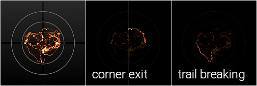
G-Map
The G-Map is a histogram of the G-Force acting on the vehicle over time.
It can be used to gauge how close to the limit a rider is riding.
Assuming a perfect world where vehicles have isotropic grip, the vehicle sufficient power and the
rider always operating it at the limit it would trace out a perfect circle, resembling the Circle of forces.
As you can see my example above is far away from that. It shows conservative riding, always staying within
the 1 g that warm track tires can easily handle. It also shows that I still have a lot to learn with regards
to consistency.
It also shows that the track in question has more right turns than left.
Future Plans
There is of course a lot more that can be done here.
The GoPro also has an accelerometer and gyro which could be integrated into the filters to yield
more accurate results.
The additional data would yield the actual lean angle which could then be used in combination with the
lateral acceleration to gauge the effectiveness of the body position/hangoff of the rider.
I also have another version of this running on a Raspberry PI coupled to an external GPS receiver.
This combination results in an all in one integrated data recording solution. One can simply connect to the
WiFi hotspot of the little computer onboard the vehicle and view the most recent sessions.
It’s rather nice because it doesn’t require the camera to be running all the time and is quite simple to use.
The drawback is that it requires fiddling together a bunch of hardware which I guess most people don’t want to deal with.
Disclaimer
There are two things that need to be said here.
First off this is not a perfect solution and even if it was it couldn’t definitely
answer the question of how close to the limit the rider is. Factors like the track surface,
weight transfer and other shenanigans are not accounted for.
Secondly, this product and/or service is not affiliated with, endorsed by or in any way associated with GoPro Inc. or its products and services. GoPro, HERO and their respective logos are trademarks or registered trademarks of GoPro, Inc.
It’s been a while since the last release but I finally finished something again.
Noise tends to eject me from my focus and flow and sometimes noise canceling headphones just aren’t enough
to prevent it.
In those instances I often mask the remaining noise with less distracting pure noise.
There already are various tools for this purpose, so there isn’t really a strict need for another one.
I just wanted to have some fun and build something that does exactly what I want and looks pretty while doing it.
As a nice bonus it gave me an opportunity to play with some more recent web technologies.
I don’t expect this to be useful to particularly many people other than myself but that’s why it’s a spare time project. :)
One of the first lessons in astrophotography is that you better find a dark place,
far away from the lights of civilization if you want to take good pictures of the night sky.
Wouldn’t it be beautiful if it was possible to photograph the Milky Way in the middle
of a city?
I wanted to try.
Step by Step
I packed my camera onto my bike and rode into night to take a few photos.
This is what they looked like after I developed them using RawTherapee.
Straigh out of camera
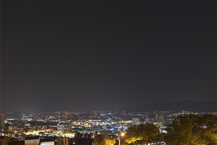
When you take a picture of the night sky in a city this is about what you will get.
At least we can see Saturn and a few stars. Let’s try to peek through the haze.
The first step is to collect more light. The more light we capture with our camera
the easier it will be to separate the photons coming from the nebulae in the galactic center from
the noise. We can gather more light by capturing more photographs.
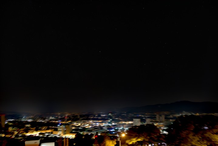
The only problem is of course that the stars are moving.
The stars are moving
We can fix this problem by aligning the images based on the stars. I used Hugin for this job.
The earth slowly turning
The next step is to combine (stack) all of the images into one.
The ground will look blurry because it moves but the stars will remain sharp.
I used Siril for this task.
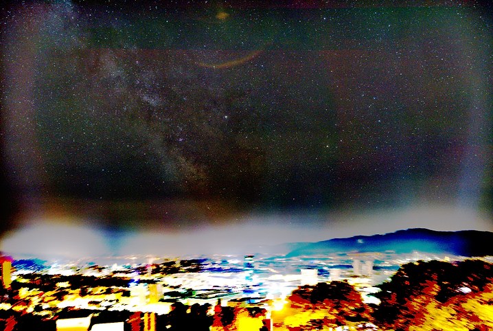
Now this is where the magic happens. We remove the ground and stars from the image
and then blur it a lot.
All this image now contains is the light pollution. Let’s subtract1 it.
With all of the light pollution gone darkness remains.
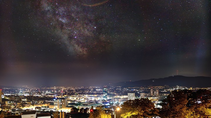
Now we can amplify the faint light in the image, increase contrast and denoise.
Finally we add the recovered light back to one of the original images and apply some final tweaks.
Why this is possible
This is possible because of two main reasons.
Light pollution is the result of light being scattered (light bouncing of particles in the air) in the air.
Unlike for instance dense smoke, light pollution does not block the light from the glowing gas clouds of the Milky Way.
This means that the signal is still there just very weak compared to the city lights.
The other reason is that the light pollution, especially higher above the horizon becomes more and more even.
That’s the property that allows us to separate it from the more focused light of the stars and nebula using a high pass filter.
Settings & Equipment
In case you are curious about the equipment and settings used:
Nikon D810, Samyang 24/1.4 @ 2.8, ISO 100, 9 pictures @ 20s, combined using winsorized sigma clipping.
Conclusions
The result is definitely noisy and not of the highest quality but still it amazes me, that this is even possible.
A consumer grade camera and free software can reveal the center of our home galaxy behind the bright haze of city lights,
showing us our place in our galaxy and the the universe beyond.
I’m curious how much farther I can push this technique with deliberately chosen framing, tweaked settings, more exposures and maybe a Didymium filter.
Further Reading
If you want to learn about astrophotography in general I recommend you to read lonelyspeck.com.
Ian is a much better writer than I will ever be and he has written a lot of great articles.
1: In practice you want to use grain extract/merge here since subtraction in most graphics software clips negative values to zero.

 View the synthwave demo
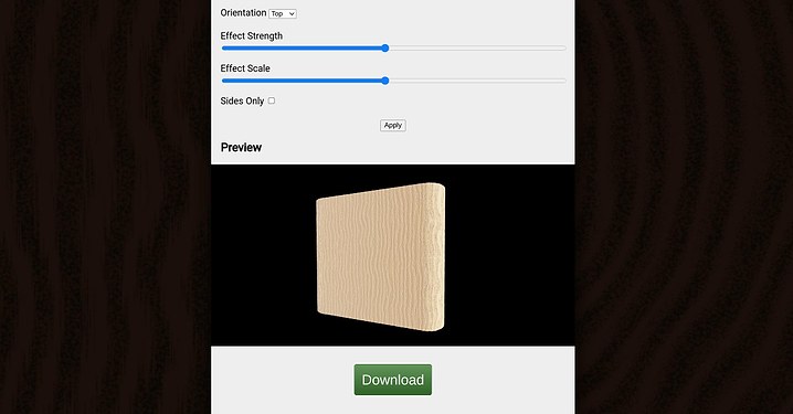 Test the 3d print texturizer
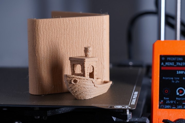 Benchy and phone stand on the prusa mini.
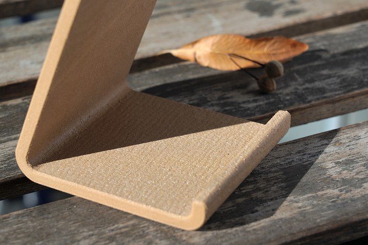 The phone stand lit by the sun.
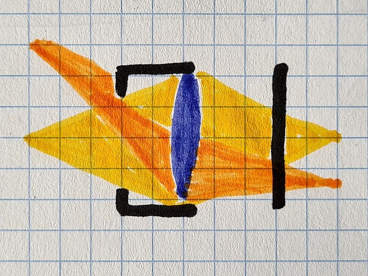 The light coming from the left (yellow, orange) is partially blocked by the lens hood (black) before hitting the lens (blue) and finally the sensor on the right (black).
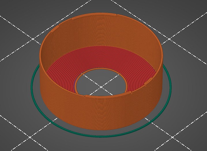 Preview of the 3D print.
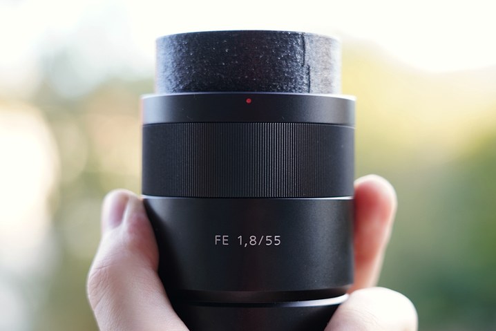 Finished product.
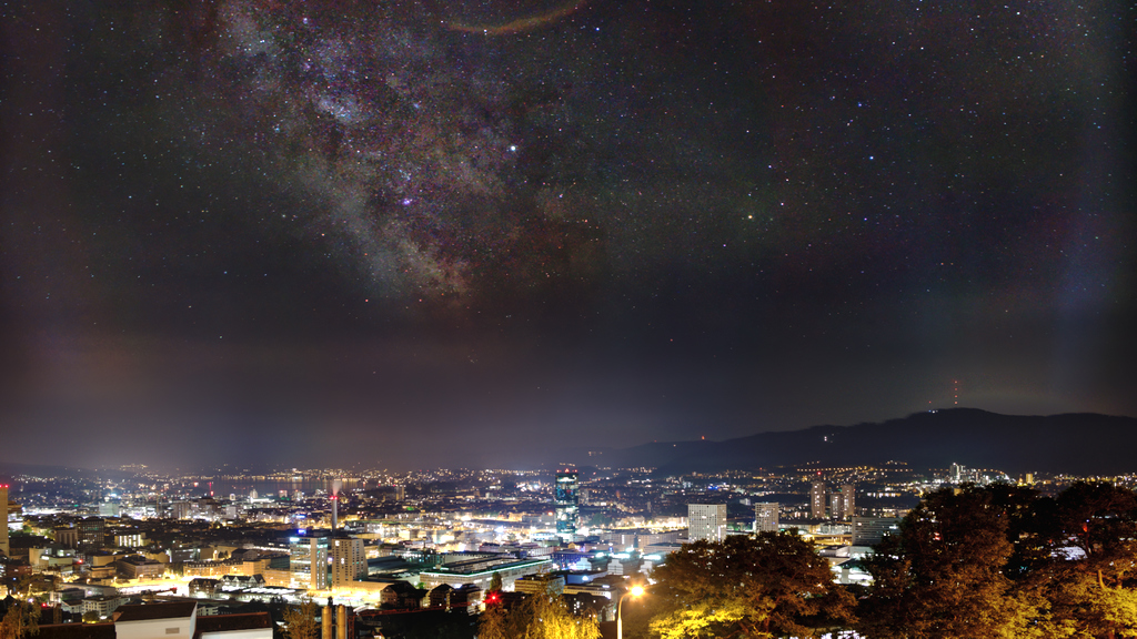
 Crop of the top right corner of some city lights at night.
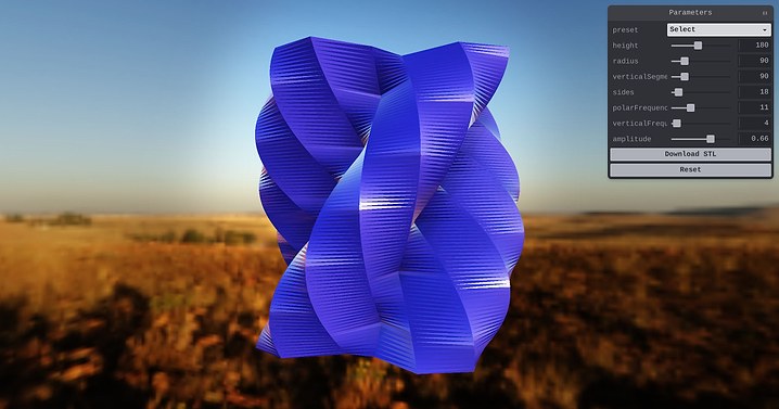 Play with generating lamp shades
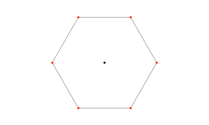

 Try the chromatic tuner
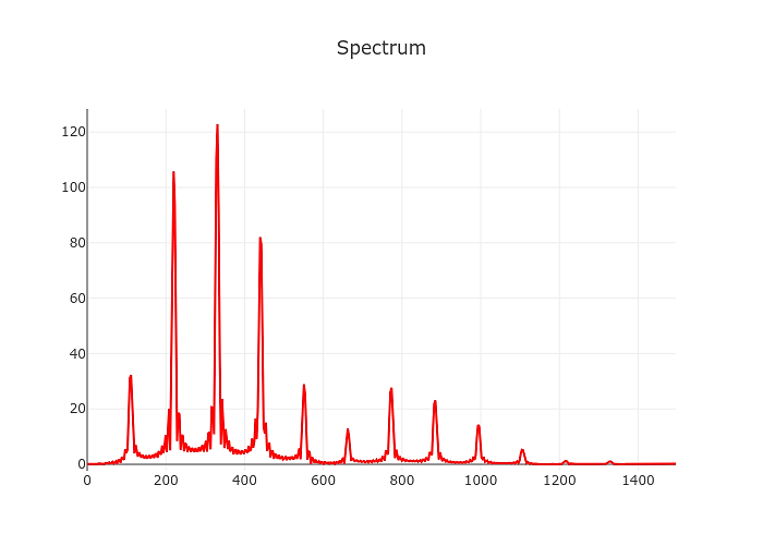
 Onset Locking
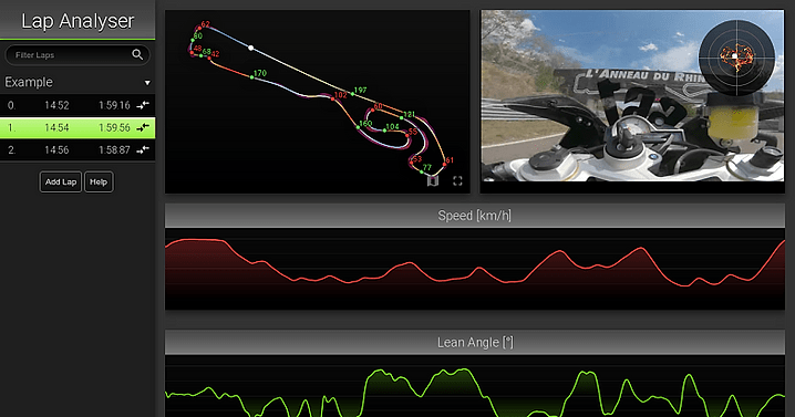 Try the lap analyser